The convolutional Neural Network architecture is central to deep learning and it is what makes possible a range of applications for computer vision, from analyzing security footage and medical imaging to enabling the automation of vehicles and machines for industry and agriculture. The scope remains unlimited.

This article provides a basic description of CNN architecture and its uses.

1. What is Convolution Neural Network

2. Build a CNN in Keras.

A. What is Convolution Neural Network

CNN is the foundation of most computer vision technologies. Unlike traditional multilayer perceptron architecture, it uses two operations called ‘convolutional’ and ‘pooling ’ to reduce an image into its essential features and uses features to understand and classify the image.

The basic building blocks of CNN are :

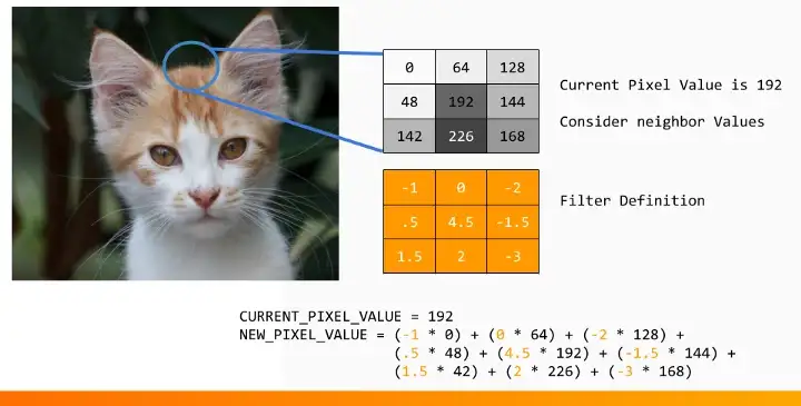
1. Convolution Layer: a ‘filter’, sometimes called a ‘kernel’, is passed over the image viewing a few pixels at a time ( for example, 3x3 and 5x5). The convolution operation is a dot product of the original pixel values with weight defined in the filter. The results are summed up into one number that represents all the pixels the filter obtained.

Consider a 5x5 whose image with varying pixel values and filter matrix whose size is 3x3 as shown in the image:

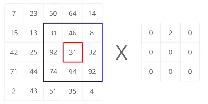
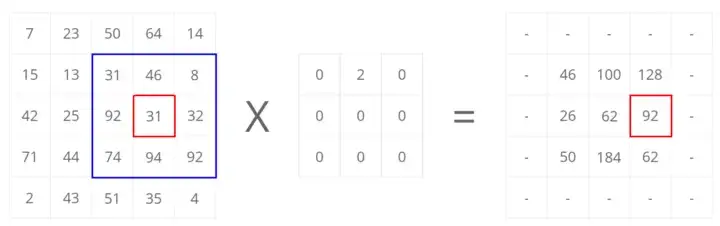
Then the convolution of the 5x5 image matrix multiplies with the 3x3 filter to output something that is called a “Feature Map”.

Formula:

An Image of matrix dimension (h x w x d), a filter (fh x fw x fd) outputs a volume of (h- fh +1) x (w- fw + 1)x 1

Example:

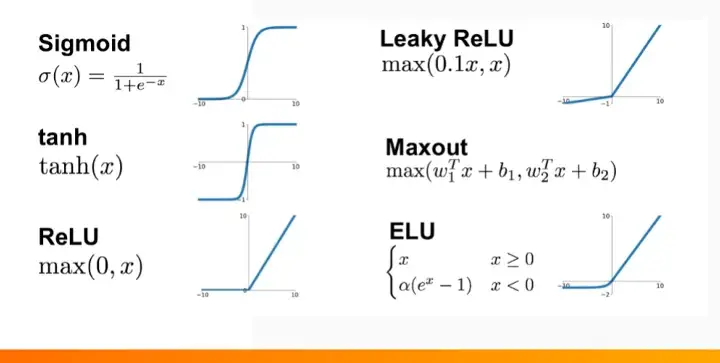
1. Activation Layer: the convolution layer generates a matrix that is much smaller in size than the original image. This matrix is run through an activation layer, which introduces non-linearity to allow the network to train itself via backpropagation.

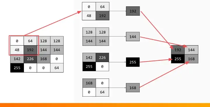
1. Pooling Layer: ‘Pooling’ is the process of further downsampling and reducing the size of the matrix. A filter is passed over the results of the previous layer and selects one number out of each group of values. This allows the network to train much faster, focusing on the most important information in each feature of the image.

   Example:

1. Fully Connected Layer: A traditional multilayer perceptron structure, its input is a one-dimensional vector representing the output of the previous layer. Its output is a list of probabilities for different possible labels attached to the image. The label that receives the highest probability is the classification decision.

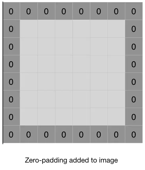
2. Padding: Sometimes filter does not fit perfectly in the input image. It leaves the border pixels, this is fine when there is very little information along the borders but a major concern when there are some features that lie within the border. For this, we use something called Padding. Padding is a simple process of adding layers of zeros to our input images so as to avoid the problems mentioned above.

B. Tutorial No 1: Building a CNN in Keras

In this tutorial, we will build a simple CNN using Keras. The network can process the standard Fashion_Mnist Dataset containing grayscale images of size 28x28 pixels associated with a label from 10 labels.

1. Defining the model: We will be using a Sequential() function which is probably the easiest way to define a deep learning model in Keras. It lets you add a layer one by one.

model = Sequential()

Use the Keras Conv2D function to create a 2-Dimensional convolution layer, with a kernel size of 3x3 pixels and a stride of 1 in the x-direction and y-direction. The Conv2D command automatically creates an activation function for you- here we are using ReLu activation.

model.add(Conv2D(32, kernel_size = (3,3),strides = (1,1),activation = ‘relu’, input_shape=(28,28,1)))

Then use the Maxpooling2D function to add a 2D max-pooling layer, with a pooling filter size of 2x2 and stride of 2 in x and y directions.

model.add(MaxPooling2D(pool_size = (2,2))

Add more convolutions and pooling this time to increase the filters to 64 filters

model.add(Conv2D(64, (5, 5), activation='relu'))
model.add(MaxPooling2D(pool_size=(2, 2)))

finally, flatten the output and define the fully connected layers that generate probabilities for ten prediction labels.

model.add(Flatten())
model.add(Dense(1000, activation='relu'))
model.add(Dense(10, activation='softmax'))

2. Compile and train the CNN:

Compile the network using the model.compile() command. Select cross-entropy loss function, Adam optimizer with learning rate 0.01, and accuracy as your metric to evaluate the performance

model.compile(loss=keras.losses.categorical_crossentropy,
              optimizer=keras.optimizers.SGD(lr=0.01),
              metrics=['accuracy'])

Now train it using model.fit(), passing the training and testing dataset and specifying your batch size and the number of epochs for training.

model.fit(x_train, y_train,
          batch_size=128,
          epochs=10,
          verbose=1,
          validation_data=(x_test, y_test),
          callbacks=[history])

3. Evaluating performance

The results look like this:

3328/60000 [>.............................] - ETA: 87s - loss: 0.2180 - acc: 0.9336
3456/60000 [>.............................] - ETA: 87s - loss: 0.2158 - acc: 0.9349
...

Use the evaluate() function to evaluate the performance of the model, using accuracy as we defined previously:

score = model.evaluate(x_test, y_test, verbose=0)
print('Test loss:', score[0])
print('Test accuracy:', score[1])